Exploring the Data
Last updated on 2025-07-01 | Edit this page
Overview
Questions
- How can I load data from CSV or TSV files into R?
- What are some functions in R that can be used to examine the data?
Objectives
- Load in our RNA-seq data files into R
- Try using some functions to explore data frames (tables) in R
- Learn how to subset parts of a data frame
Getting started with the data
In this tutorial, we will learn some R through creating plots to visualise data from an RNA-seq experiment.
The GREIN platform (GEO RNA-seq Experiments Interactive Navigator) provides >6,500 published datasets from GEO that have been uniformly processed. It is available at http://www.ilincs.org/apps/grein/. You can search for a dataset of interest using the GEO code. GREIN provide QC metrics for the RNA-seq datasets and both raw and normalized counts. We will use the normalized counts here. These are the counts of reads for each gene for each sample normalized for differences in sequencing depth and composition bias. Generally, the higher the number of counts the more the gene is expressed.
RNA-seq dataset from Fu et al.
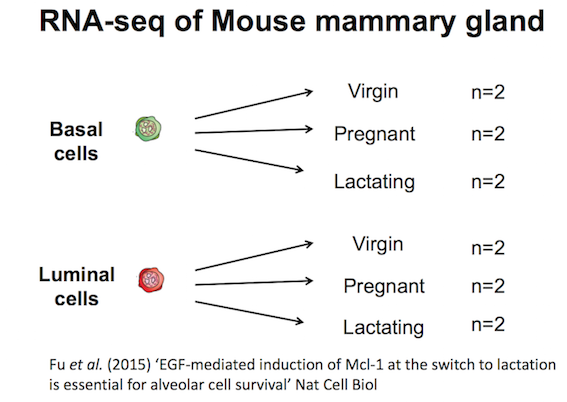
Here we will create some plots using RNA-seq data from the paper by Fu et al. 2015 (GEO accession number GSE60450). Mice, like all mammals, have mammary glands which produce milk to nourish their young. The authors of this study were interested in examining how the mammary epithelium (which line the mammary glands) expands and develops during pregnancy and lactation.
This study examined expression in basal and luminal cells from mice at different stages (virgin, pregnant and lactating). Basal cells are mammary stem cells and luminal cells secrete milk. There are 2 samples per group and 6 groups, so 12 samples in total.
Tidyverse

The tidyverse package that we installed previously is a
collection of R packages that includes the extremely widely used
ggplot2 package.
The tidyverse makes data science faster, easier and more fun.
Tidyverse is built on the principle of organizing data in a tidy format.
Data files
Your turn 2.1
If you haven’t already downloaded the data.zip file for this workshop, you can click here to download it now.
Unzip the file and store the extracted data folder in
your working directory.
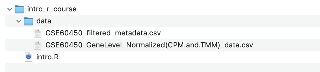
Make sure the data is in the correct directory
Inside your current working directory directory
(e.g. intro_r_course), there should be a directory called
data and inside that directory should be two CSV files.
In the next section, you will load these files into R using the file path (i.e. where they are located in the filesystem), so the code in this tutorial expects the files to be in the above location. If you have the files in a different location, you also have the option of changing the commands in the following sections to match where the files are located on your computer.
Loading the data
We use library() to load in the packages that we need.
As described in the cooking analogy in the first screenshot,
install.packages() is like buying a saucepan,
library() is taking it out of the cupboard to use it.
Your turn 2.2
Load in the tidyverse package using the library()
function:
R
library(tidyverse)
The files we will use are CSV comma-separated, so we will use the
read_csv() function from the tidyverse. There is also a
read_tsv() function for tab-separated values.
We will use the counts file called
GSE60450_GeneLevel_Normalized(CPM.and.TMM)_data.csv that’s
in a folder called data i.e. the path to the file should be
data/GSE60450_GeneLevel_Normalized(CPM.and.TMM)_data.csv.
We can read the counts file into R with the command below. We’ll
store the contents of the counts file in an object
called counts. This stores the file contents in R’s memory
making it easier to use.
Your turn 2.3
Load the count data into R. We will store the contents of the counts
file in an object called counts. Note that
we need to put quotes (““) around file paths.
R
# Read in counts file
counts <- read_csv("data/GSE60450_GeneLevel_Normalized(CPM.and.TMM)_data.csv")
OUTPUT
New names:
Rows: 23735 Columns: 14
── Column specification
──────────────────────────────────────────────────────── Delimiter: "," chr
(2): ...1, gene_symbol dbl (12): GSM1480291, GSM1480292, GSM1480293,
GSM1480294, GSM1480295, GSM148...
ℹ Use `spec()` to retrieve the full column specification for this data. ℹ
Specify the column types or set `show_col_types = FALSE` to quiet this message.
• `` -> `...1`
Note: In R, structured tables like these are called data frames.
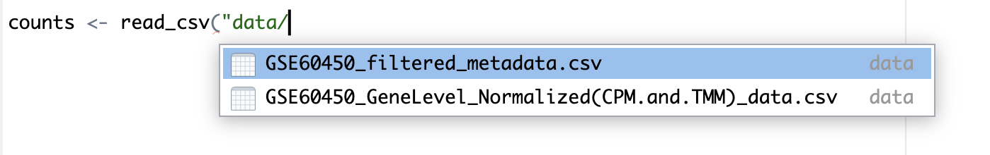
Tab completion for file paths
We mentioned tab completion in the previous section, but tab completion can also complete file paths. This means you don’t have to type out the long filenames in the codeblock above, but instead, begin to type out a few characters, then press tab and see the autocompletion options.
No need to be overwhelmed by the outputs! It contains information
regarding “column specification” (telling us that there is a missing
column name in the header and it has been filled with the name “…1”,
which is how read_csv handles missing column names by default). We will
fix this later. It also tells us what data types read_csv
is detecting in each column. Columns with text characters have been
detected (col_character) and also columns with numbers
(col_double). We won’t get into the details of R data types
in this tutorial but they are important to know when you get more
proficient in R. You can read more about them in the R
for Data Science book.
Your turn 2.4
Load the sample information data into R. We will store the contents
of this file in an object called sampleinfo.
R
# Read in metadata
sampleinfo <- read_csv("data/GSE60450_filtered_metadata.csv")
OUTPUT
New names:
Rows: 12 Columns: 4
── Column specification
──────────────────────────────────────────────────────── Delimiter: "," chr
(4): ...1, characteristics, immunophenotype, developmental stage
ℹ Use `spec()` to retrieve the full column specification for this data. ℹ
Specify the column types or set `show_col_types = FALSE` to quiet this message.
• `` -> `...1`
It is very common when looking at biological data that you have two
types of data. One is the actual data (in this case, our
counts object, which has the expression values of different
genes in each sample). The other is metadata
i.e. information about our samples (in this case, our
sampleinfo object includes information about whether
samples are from basal or luminal cells and whether the cells were from
mice which are virgin/pregnant/lactating, etc.)
What data have we imported into R?
To summarise, we have imported two data frames (i.e. tables) into R:
-
countsobject is our gene expression data -
sampleinfoobject is our sample metadata
Your turn 2.5
Let’s get used to making some mistakes in R, so we know what errors look like and how to handle them.
Test what happens if you type
Library(tidyverse)
What is wrong and how would you fix it?Test what happens if you type
library(tidyverse
What is wrong and how would you fix it?Test what happens if you type
read_tsv("data/GSE60450_filtered_metadata.csv")
What is wrong and how would you fix it?Test what happens if you type
read_csv("data/GSE60450_filtered_metadata.csv)
What is wrong and how would you fix it?Test what happens if you type
read_csv("GSE60450_filtered_metadata.csv")
What is wrong and how would you fix it?
Don’t forget you can press ESC to escape the current command and start a new prompt.
Getting to know the data
When assigning a value to an object, R does not print the value. We
do not see what is in counts or sampleinfo.
But there are ways we can look at the data.
Your turn 2.6
Click on the sampleinfo object in your global
environment panel on the right-hand-side of RStudio. This will open a
new tab.
This is the equivalent of using the View() function.
e.g.
R
View(sampleinfo)
Your turn 2.7
Type the name of the object and this will print the first few lines and some information, such as number of rows. Note that this is similar to how we looked at the value of objects we assigned in the previous section.
R
sampleinfo
OUTPUT
# A tibble: 12 × 4
   ...1       characteristics              immunophenotype `developmental stage`
   <chr>      <chr>                        <chr>           <chr>
 1 GSM1480291 mammary gland, luminal cell… luminal cell p… virgin
 2 GSM1480292 mammary gland, luminal cell… luminal cell p… virgin
 3 GSM1480293 mammary gland, luminal cell… luminal cell p… 18.5 day pregnancy
 4 GSM1480294 mammary gland, luminal cell… luminal cell p… 18.5 day pregnancy
 5 GSM1480295 mammary gland, luminal cell… luminal cell p… 2 day lactation
 6 GSM1480296 mammary gland, luminal cell… luminal cell p… 2 day lactation
 7 GSM1480297 mammary gland, basal cells,… basal cell pop… virgin
 8 GSM1480298 mammary gland, basal cells,… basal cell pop… virgin
 9 GSM1480299 mammary gland, basal cells,… basal cell pop… 18.5 day pregnancy
10 GSM1480300 mammary gland, basal cells,… basal cell pop… 18.5 day pregnancy
11 GSM1480301 mammary gland, basal cells,… basal cell pop… 2 day lactation
12 GSM1480302 mammary gland, basal cells,… basal cell pop… 2 day lactation
We can also take a look the first few lines with head().
This shows us the first 6 lines.
Your turn 2.8
Use head() to look at the first few lines of
counts.
R
head(counts)
OUTPUT
# A tibble: 6 × 14
  ...1        gene_symbol GSM1480291 GSM1480292 GSM1480293 GSM1480294 GSM1480295
  <chr>       <chr>            <dbl>      <dbl>      <dbl>      <dbl>      <dbl>
1 ENSMUSG000… Gnai3          243.      256.         240.       217.       84.7
2 ENSMUSG000… Pbsn             0         0            0          0         0
3 ENSMUSG000… Cdc45           11.2      13.8         11.6        4.27      8.35
4 ENSMUSG000… H19              6.31      8.53         7.09      11.0       0.194
5 ENSMUSG000… Scml2            2.19      4.66         2.80       2.50      1.24
6 ENSMUSG000… Apoh             0.224     0.0840       0          0         0
# ℹ 7 more variables: GSM1480296 <dbl>, GSM1480297 <dbl>, GSM1480298 <dbl>,
#   GSM1480299 <dbl>, GSM1480300 <dbl>, GSM1480301 <dbl>, GSM1480302 <dbl>
We can also look at the last few lines with tail(). This
shows us the last 6 lines. This can be useful to check the bottom of the
file, that it looks ok.
Your turn 2.6
Use tail() to look at the last few lines of
counts.
R
tail(counts)
OUTPUT
# A tibble: 6 × 14
  ...1        gene_symbol GSM1480291 GSM1480292 GSM1480293 GSM1480294 GSM1480295
  <chr>       <chr>            <dbl>      <dbl>      <dbl>      <dbl>      <dbl>
1 ENSMUSG000… Pcdha7           0.134     0          0            0          0
2 ENSMUSG000… Gm34240          0         0          0            0          0
3 ENSMUSG000… Pcdhga3          0.582     2.27       0.334        1.10       0
4 ENSMUSG000… Gm20750          0         0.0840     0.0417       0          0
5 ENSMUSG000… Rhbg             5.28      4.96       6.26         3.98       1.01
6 ENSMUSG000… Mat2a          212.      225.        97.9         70.1       22.0
# ℹ 7 more variables: GSM1480296 <dbl>, GSM1480297 <dbl>, GSM1480298 <dbl>,
#   GSM1480299 <dbl>, GSM1480300 <dbl>, GSM1480301 <dbl>, GSM1480302 <dbl>
Your turn 2.7
What are the cell types of the first 6 samples in the metadata for the Fu et al. 2015 experiment?
R
head(sampleinfo)
OUTPUT
# A tibble: 6 × 4
  ...1       characteristics               immunophenotype `developmental stage`
  <chr>      <chr>                         <chr>           <chr>
1 GSM1480291 mammary gland, luminal cells… luminal cell p… virgin
2 GSM1480292 mammary gland, luminal cells… luminal cell p… virgin
3 GSM1480293 mammary gland, luminal cells… luminal cell p… 18.5 day pregnancy
4 GSM1480294 mammary gland, luminal cells… luminal cell p… 18.5 day pregnancy
5 GSM1480295 mammary gland, luminal cells… luminal cell p… 2 day lactation
6 GSM1480296 mammary gland, luminal cells… luminal cell p… 2 day lactation
The first 6 samples are luminal cells.
Dimensions of the data
You can print the number of rows and columns using the function
dim().
For example:
R
dim(sampleinfo)
OUTPUT
[1] 12 4sampleinfo has 12 rows, corresponding to our 12 samples,
and 4 columns, corresponding to different features about the
samples.
Tip: Always Verify Your Data Size
Double-check that your data has the expected number of rows and columns. It’s easy to read the wrong file or encounter corrupted downloads. Catching these issues early will save you a lot of trouble later!
Your turn 2.8
Check how many rows and columns are in counts. Do these
numbers match what we expected?
R
dim(counts)
OUTPUT
[1] 23735 14We know that there are 12 samples in our data (see the diagram above), and we don’t know how many genes were measured.
Rows: 23735. This means there are 23735 genes, which could be correct (we didn’t know how many genes were measured).
Columns: 14. We would expect to have 12 columns
corresponding to our 12 samples, but instead we have 14. Why is this?
Have a look back at when we visualised the counts data,
there are two extra columns in the data corresponding to gene IDs and
gene names.
In the Environment Tab in the top right panel in RStudio we can also see the number of rows and columns in the objects we have in our session.
Column and row names of the data
Your turn 2.9
Check the column and row names used in in sampleinfo
R
colnames(sampleinfo)
rownames(sampleinfo)
Subsetting
Subsetting is very useful tool in R which allows you to extract parts of the data you want to analyse. There are multiple ways to subset data and here we’ll only cover a few.
We can use the $ operator to access individual columns
by name.
Your turn 2.10
Extract the ‘immunophenotype’ column of the metadata.
R
sampleinfo$immunophenotype
We can also use square brackets [ ] to access the rows
and columns of a matrix or a table.
For example, we can extract the first row ‘1’ of the data, using the number on the left-hand-side of the comma.
Your turn 2.11
Extract the first row using square brackets.
R
sampleinfo[1,]
Here we extract the second column ‘2’ of the data, as indicated on the right-hand-side of the comma.
Your turn 2.12
Extract the second column using square brackets.
R
sampleinfo[,2]
You can use a combination of number of row and column to extract one element in the matrix.
Your turn 2.13
Extract the element in the first row and second column.
R
sampleinfo[1,2]
Your turn 2.14
We can also subset using a range of numbers. For example, if we
wanted the first three rows of sampleinfo
R
sampleinfo[1:3,]
Or if we wanted the 2nd, 4th, and 5th row:
R
sampleinfo[c(2,4,5),]
The c() function
We use the c() function extremely often in R when we
have multiple items that we are combining (‘c’ stands for
concatenating). We will see it again in this tutorial.
Renaming column names
In the previous section, when we loaded in the data from the csv file, we noticed that the first column had a missing column name and by default, read_csv function assigned a name of “...1” to it. Let’s change this column to something more descriptive now. We can do this by combining a few things we’ve just learnt.
Your turn 2.15
First, we use the colnames() function to obtain the
column names of sampleinfo. Then we use square brackets to subset the
first value of the column names ([1]). Last, we use the
assignment operator (<-) to set the new value of the
first column name to “sample_id”.
R
colnames(sampleinfo)[1] <- "sample_id"
Let’s check if this has been changed correctly.
R
sampleinfo
OUTPUT
# A tibble: 12 × 4
   sample_id  characteristics              immunophenotype `developmental stage`
   <chr>      <chr>                        <chr>           <chr>
 1 GSM1480291 mammary gland, luminal cell… luminal cell p… virgin
 2 GSM1480292 mammary gland, luminal cell… luminal cell p… virgin
 3 GSM1480293 mammary gland, luminal cell… luminal cell p… 18.5 day pregnancy
 4 GSM1480294 mammary gland, luminal cell… luminal cell p… 18.5 day pregnancy
 5 GSM1480295 mammary gland, luminal cell… luminal cell p… 2 day lactation
 6 GSM1480296 mammary gland, luminal cell… luminal cell p… 2 day lactation
 7 GSM1480297 mammary gland, basal cells,… basal cell pop… virgin
 8 GSM1480298 mammary gland, basal cells,… basal cell pop… virgin
 9 GSM1480299 mammary gland, basal cells,… basal cell pop… 18.5 day pregnancy
10 GSM1480300 mammary gland, basal cells,… basal cell pop… 18.5 day pregnancy
11 GSM1480301 mammary gland, basal cells,… basal cell pop… 2 day lactation
12 GSM1480302 mammary gland, basal cells,… basal cell pop… 2 day lactation
The first column is now named “sample_id”.
We can also do the same to the counts data. This time, we rename the first column name from “...1” to “gene_id”.
Your turn 2.16
R
colnames(counts)[1] <- "gene_id"
Note: there are multiple ways to rename columns. We’ve covered one
way here, but another way is using the rename() function.
When programming, you’ll often find many ways to do the same thing.
Often there is one obvious method depending on the context you’re
in.
Structure and Summary
Other useful commands for checking data are str() and
summary().
str() shows us the structure of our data. It shows us
what columns there are, the first few entries, and what data type they
are e.g. character or numbers (double or integer).
R
str(sampleinfo)
OUTPUT
spc_tbl_ [12 × 4] (S3: spec_tbl_df/tbl_df/tbl/data.frame)
 $ sample_id          : chr [1:12] "GSM1480291" "GSM1480292" "GSM1480293" "GSM1480294" ...
 $ characteristics    : chr [1:12] "mammary gland, luminal cells, virgin" "mammary gland, luminal cells, virgin" "mammary gland, luminal cells, 18.5 day pregnancy" "mammary gland, luminal cells, 18.5 day pregnancy" ...
 $ immunophenotype    : chr [1:12] "luminal cell population" "luminal cell population" "luminal cell population" "luminal cell population" ...
 $ developmental stage: chr [1:12] "virgin" "virgin" "18.5 day pregnancy" "18.5 day pregnancy" ...
 - attr(*, "spec")=
  .. cols(
  ..   ...1 = col_character(),
  ..   characteristics = col_character(),
  ..   immunophenotype = col_character(),
  ..   `developmental stage` = col_character()
  .. )
 - attr(*, "problems")=<externalptr>
summary() generates summary statistics of our data. For
numeric columns (columns of type double or integer) it outputs
statistics such as the min, max, mean and median. We will demonstrate
this with the counts file as it contains numeric data. For character
columns it shows us the length (how many rows).
R
summary(counts)
OUTPUT
   gene_id          gene_symbol          GSM1480291          GSM1480292
 Length:23735       Length:23735       Min.   :    0.000   Min.   :    0.000
 Class :character   Class :character   1st Qu.:    0.000   1st Qu.:    0.000
 Mode  :character   Mode  :character   Median :    1.745   Median :    1.891
                                       Mean   :   42.132   Mean   :   42.132
                                       3rd Qu.:   29.840   3rd Qu.:   29.604
                                       Max.   :12525.066   Max.   :12416.211
   GSM1480293          GSM1480294          GSM1480295
 Min.   :    0.000   Min.   :    0.000   Min.   :0.000e+00
 1st Qu.:    0.000   1st Qu.:    0.000   1st Qu.:0.000e+00
 Median :    0.918   Median :    0.888   Median :5.830e-01
 Mean   :   42.132   Mean   :   42.132   Mean   :4.213e+01
 3rd Qu.:   21.908   3rd Qu.:   19.921   3rd Qu.:1.227e+01
 Max.   :49191.148   Max.   :55692.086   Max.   :1.119e+05
   GSM1480296          GSM1480297          GSM1480298
 Min.   :0.000e+00   Min.   :    0.000   Min.   :    0.000
 1st Qu.:0.000e+00   1st Qu.:    0.000   1st Qu.:    0.000
 Median :5.440e-01   Median :    2.158   Median :    2.254
 Mean   :4.213e+01   Mean   :   42.132   Mean   :   42.132
 3rd Qu.:1.228e+01   3rd Qu.:   27.414   3rd Qu.:   26.450
 Max.   :1.087e+05   Max.   :10489.311   Max.   :10662.486
   GSM1480299          GSM1480300          GSM1480301
 Min.   :    0.000   Min.   :    0.000   Min.   :    0.000
 1st Qu.:    0.000   1st Qu.:    0.000   1st Qu.:    0.000
 Median :    1.854   Median :    1.816   Median :    1.629
 Mean   :   42.132   Mean   :   42.132   Mean   :   42.132
 3rd Qu.:   24.860   3rd Qu.:   23.443   3rd Qu.:   23.444
 Max.   :15194.048   Max.   :17434.935   Max.   :19152.728
   GSM1480302
 Min.   :    0.000
 1st Qu.:    0.000
 Median :    1.749
 Mean   :   42.132
 3rd Qu.:   24.818
 Max.   :15997.193
Key Points
- The
read_csv()andread_tsv()functions can be used to load in CSV and TSV files in R - The
head()andtail()functions can print the first and last parts of an object and thedim()function prints the dimensions of an object - Subsetting can be done with the
$operator using column names or using square brackets[ ] - The
str()andsummary()functions are useful functions to get an overview or summary of the data