![]()
![]()
Introduction to Variant Calling using Galaxy
Overview
This tutorial is designed to introduce the tools, data types and workflow of variant detection. We will align reads to the genome, look for differences between reads and reference genome sequence, and filter the detected genomic variation manually to understand the computational basis of variant calling.
We cover the concepts of detecting small variants (SNVs and indels) in human genomic DNA using a small set of reads from chromosome 22.
Learning Objectives
At the end of the course, you will be able to:
- Work with the FASTQ format and base quality scores
- Align reads to generate a BAM file and subsequently generate a pileup file
- Run the FreeBayes variant caller to find SNVs and indels
- Visualise BAM files using the Integrative Genomics Viewer (IGV) and identify likely SNVs and indels by eye
Requirements
This workshop uses Galaxy as a platform. It is recommended that participants who have not used Galaxy before either sign up for our Intro to GVL workshop, or work through this tutorial themselves beforehand.
This is a hands-on workshop and attendees are required to bring their own laptops.
Background
Some background reading material - background
Where is the data in this tutorial from?
The workshop is based on analysis of short read data from the exome of chromosome 22 of a single human individual. There are one million 76bp reads in the dataset, produced on an Illumina GAIIx from exome-enriched DNA. This data was generated as part of the 1000 genomes Genomes project.
1. Preparation
- Make sure you have an instance of Galaxy ready to go.
- For example, you can use the Galaxy Australia server.
- Create a new history for this tutorial.
- In the history pane, click on the cog icon at the top right.
- Click Create New.
- Click on Unnamed history and re-name it.
- Import data for the tutorial.
- In this case, we are uploading a FASTQ file.
- Method 1
Paste/Fetch data from a URL to Galaxy.- In the Galaxy tools panel (left), click on
Get Dataand chooseUpload File. - Click Paste/Fetch data and paste the following URL into the box
- In the Galaxy tools panel (left), click on
1 2 3 4 5 6 7 8 9 10 11 | |
Summary:
So far, we have started a Galaxy instance, got hold of our data and uploaded it to
the Galaxy instance.
Now we are ready to perform our analysis.
2. Quality Control
The first step is to evaluate the quality of the raw sequence data. If the quality is poor, then adjustments can be made - e.g. trimming the short reads, or adjusting your expectations of the final outcome!
1. Take a look at the FASTQ file
Click on the eye icon to the top right of the FASTQ file to view the a snippet of the file.
Note that each read is represented by 4 lines: * read identifier * short read sequence * separator * short read sequence quality scores
e.g.
identifier:    @61CC3AAXX100125:7:72:14903:20386/1
read sequence: TTCCTCCTGAGGCCCCACCCACTATACATCATCCCTTCATGGTGAGGGAGACTTCAGCCCTCAATGCCACCTTCAT
separator:     +
quality score: ?ACDDEFFHBCHHHHHFHGGCHHDFDIFFIFFIIIIHIGFIIFIEEIIEFEIIHIGFIIIIIGHCIIIFIID?@<6
For more details see FASTQ.
2. Assessing read quality from the FASTQ files
- From the Galaxy tools panel, in the search box at the top, type in “FastQC”.
- Click on
FastQC
The input FASTQ file will be selected by default. Keep the other defaults and click execute.
Tip: Note the batch processing interface of Galaxy:
- grey = waiting in queue
- yellow = running
- green = finished
- red = tried to run and failed
When the job has finished, click on the eye icon to view the newly generated data (in this case a set of quality metrics for the FASTQ data). This will be a file called FastQC on data 1: Web page. Look at the various quality scores. The data looks pretty good - high Per base sequence quality (avg. above 30).
3. Alignment to the reference - (FASTQ to BAM)
The basic process here to map individual reads - from the input sample FASTQ file - to a matching region on the reference genome.
1. Align the reads with BWA
We will map (align) the reads with the BWA tool to the human reference genome. For this tutorial, use Human reference genome 19 (hg19) - this is hg19 from UCSC.
-
Align the reads [3-5mins]: from the Galaxy tools panel, search for
Map with BWA-MEM
From the options:- Will you selection a reference genome…: Use a built-in genome index
- Using reference genome: set to hg19
- Single or Paired-end reads: set to Single
- Make sure your fastq file is the input file.
- Keep other options as default and click execute.
Note: This is the longest step in the workshop and will take a few minutes, possibly more depending on how many people are also scheduling mappings
-
Sort the BAM file: from the Galaxy tools panel, search for
SortSam
From the options:- Set the input file to be the output BAM file from the previous step.
- Sort by: set to Coordinate
- Keep other options as default and click execute
2. Examine the alignment
-
To examine the output sorted BAM file, we need to first convert it into readable SAM format. From the Galaxy tools panel, search for
BAM-to-SAM
From the options:- BAM File to Convert: select your sorted BAM file
- Keep all options as default and click execute
-
Examine the generated Sequence Alignment Map (SAM) file.
- Click the eye icon in the History pane next to the newly generated file
- Familiarise yourself with the SAM format
- Note that some reads have mapped to non-chr22 chromosomes (see column 3).
This is the essence of alignment algorithms - the aligner does the best it can, but because of compromises in accuracy vs performance and repetitive sequences in the genome, not all the reads will necessarily align to the ‘correct’ sequence or could this be suggesting the presence of a structural variant?
This can be done as follows:
Click on the pencil icon (edit attributes) and change Name e.g. Sample.bam or Sample.sam or Sample.sorted.bam etc.
3. Assess the alignment data
We can generate some mapping statistics from the BAM file to assess the quality of our alignment.
-
Run IdxStats. From the Galaxy tools panel, search for the tool
IdxStats - Select the sorted BAM file as input.
- Keep other options as default and click execute.
IdxStats generates a tab-delimited output with four columns. Each line consists of a reference sequence name (e.g. a chromosome), reference sequence length, number of mapped reads and number of placed but unmapped reads.
We can see that most of the reads are aligning to chromosome 22 as expected.
-
Run Flagstat. From the Galaxy tools panel, search for
Flagstat - Select the sorted BAM file as input.
- Keep other options as default and click execute.
Note that in this case the statistics are not very informative. This is because the dataset has been generated for this workshop and much of the noise has been removed (and in fact we just removed a lot more noise in the previous step); also we are using single ended read data rather than paired-end so some of the metrics are not relevant.
4. Visualise the BAM file with IGV
To visualise the alignment data:
- Click on the sorted BAM file dataset in the History panel.
- Click on “Display with IGV web current”. This should download a .jnlp Java Web Start file to your computer. Open this file to run IGV. (You will need Java installed on your computer to run IGV). NOTE: If IGV is already open on your computer, you can click “local” instead of “web current”, and this will open the BAM file in your current IGV session.
- Once IGV opens, it will show you the BAM file. This may take a bit of time as the data is downloaded.
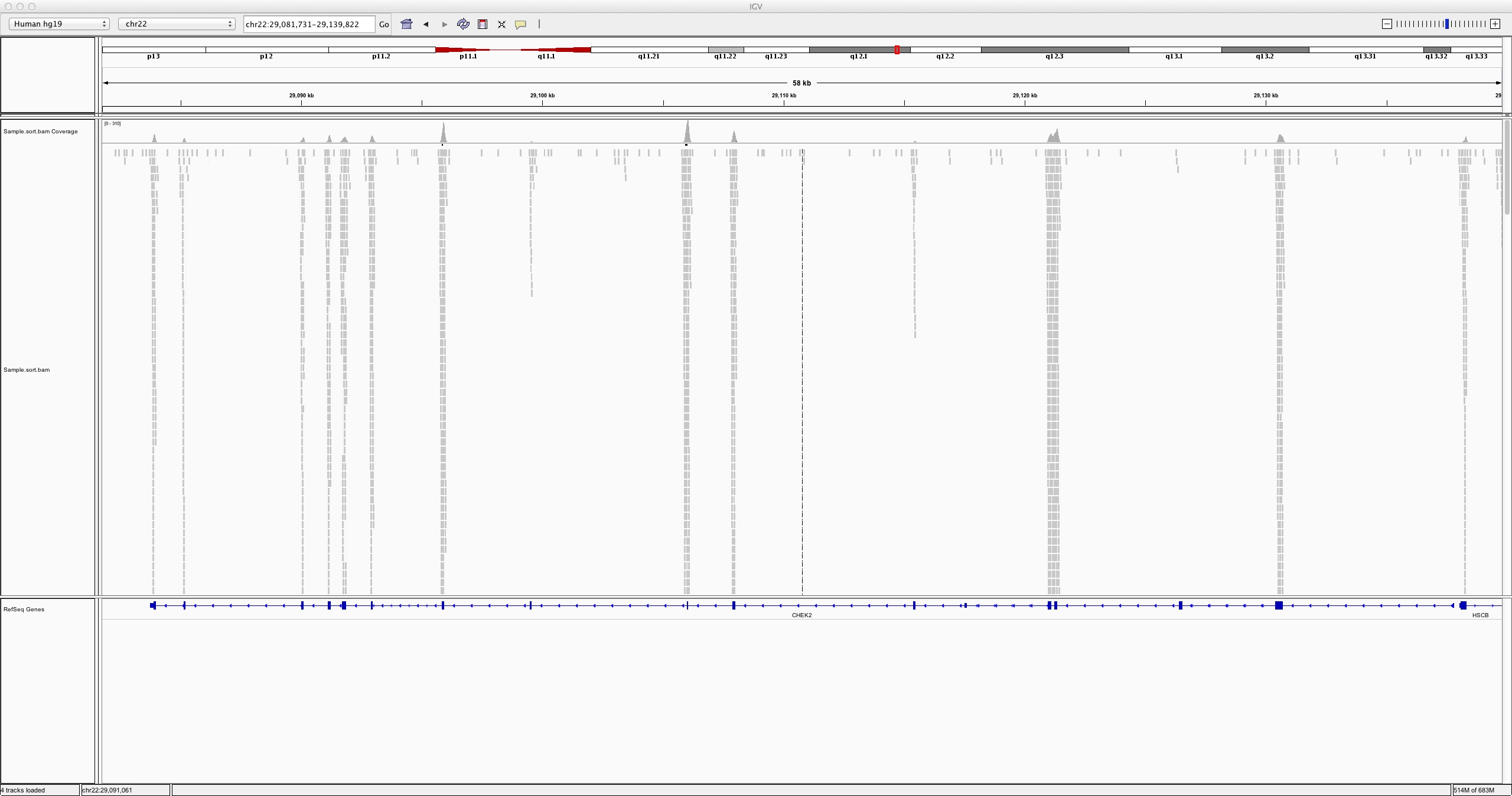
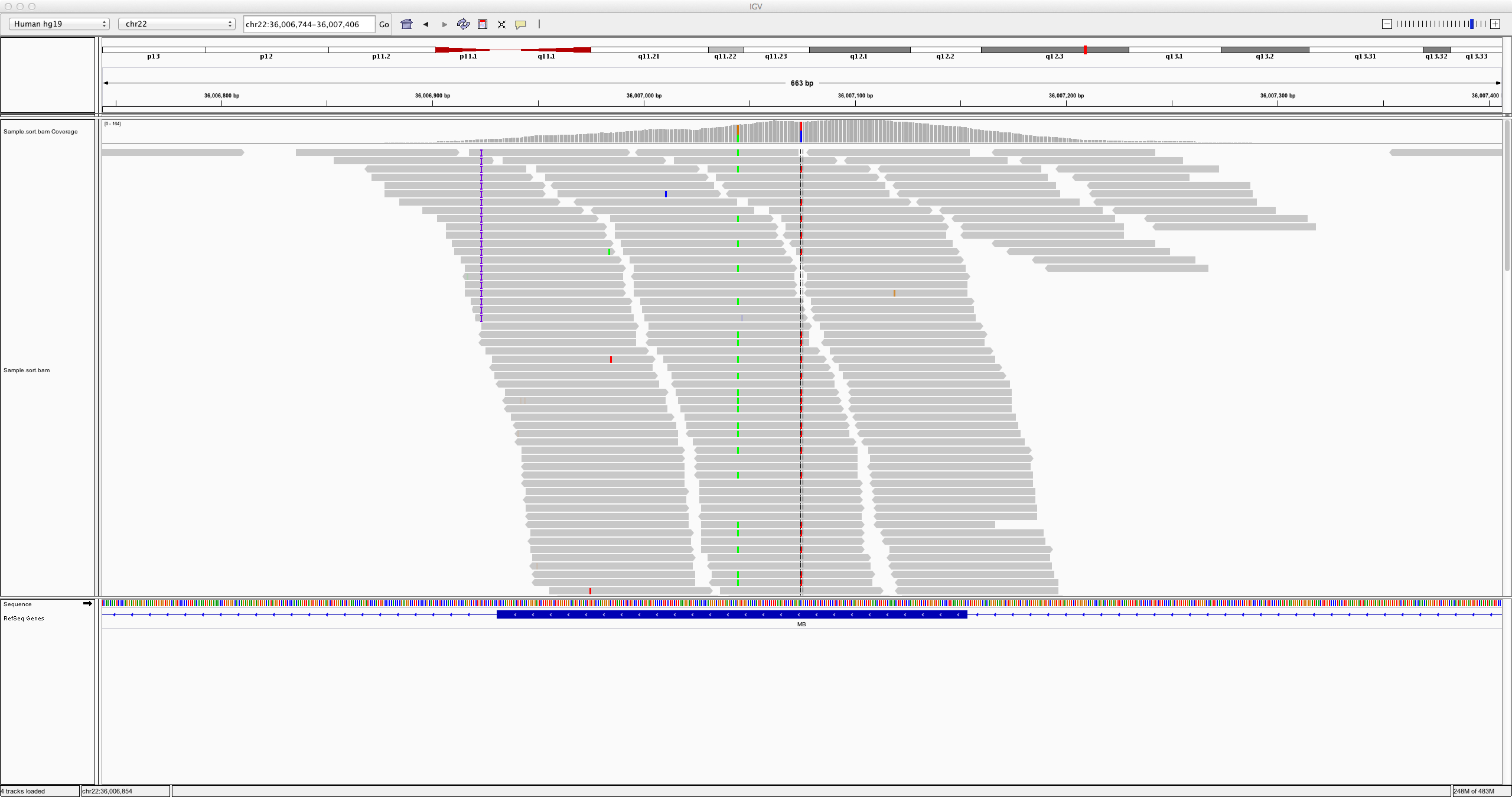
- Our reads for this tutorial are from chromosome 22, so select chr22 from the second drop box under the toolbar. Zoom in to view alignments of reads to the reference genome.
Try looking at region chr22:36,006,744-36,007,406
Can you see a few variants?
Don’t close IGV yet as we’ll be using it later.
5. Generate a pileup file
A pileup is essentially a column-wise representation of the aligned reads - at the base level - to the reference. The pileup file summarises all data from the reads at each genomic region that is covered by at least one read. Each row of the pileup file gives similar information to a single vertical column of reads in the IGV view.
The current generation of variant calling tools do not output pileup files, and you don’t need to do this section in order to use FreeBayes in the next section. However, a pileup file is a good illustration of the evidence the variant caller is looking at internally, and we will produce one to see this evidence.
1. Generate a pileup file
From the Galaxy tools panel, search for
From the options:
- Call consensus according to MAQ model: set to Yes
This generates a called ‘consensus base’ for each chromosomal position. This would allow us to use this pileup directly for variant detection, if we wanted. - Keep other options as default and click execute
Galaxy tries to assign a datatype attribute to every output file. In this case, you’ll need to manually set the datatype to pileup.
- First, rename the output to something more meaningful by clicking on the pencil icon
- To change the datatype, click on the Datatype link from the top tab while you’re editing attributes.
- For downstream processing we want to tell Galaxy that this is a pileup file. From the drop-down, select Pileup and click save.
* 1. chromosome
* 2. position
* 3. current reference base
* 4. consensus base from the mapped reads
* 5. consensus quality
* 6. SNV quality
* 7. maximum mapping quality
* 8. coverage
* 9. bases within reads
* 10. quality valuesFurther information on (9):
Each character represents one of the following (the longer this string, higher the coverage):
- . = match on forward strand for that base
- , = match on reverse strand
- ACGTN = mismatch on forward
- acgtn = mismatch on reverse
- +[0-9]+[ACGTNacgtn]+’ = insertion between this reference position and the next
- -[0-9]+[ACGTNacgtn]+’ = deletion between this reference position and the next
- ^ = start of read
- $ = end of read
- BaseQualities = one character per base in ReadBases, ASCII encoded Phred scores
2. Filter the pileup file
If you click the eye icon to view the contents of your pileup file, you’ll see that the visible rows of the file aren’t very interesting as they are outside chromosome 22 and have very low coverage. Let’s filter to regions with coverage of at least 10 reads.
From the Galaxy tools panel, search for
From the options:
- which contains: set to Pileup with ten columns (with consensus). This is to match the Call consensus according to MAQ model option we selected earlier - the filter tool needs to know to expect the 10-column rather than 6-column format.
- Do not report positions with coverage lower than: set to 10
Try this filtering step two ways:
- First, set the parameter Only report variants? to No. This will give you all locations with a coverage of at least 10 and sufficient read quality. This is similar to the information you see when you look at IVG: each pilup row corresponds to a column of aligned bases at one genomic location.
- Then, repeat the step but set Only report variants? to Yes. This will effectively do variant calling: it will give you only locations that have some evidence that there might be a variant present. This variant calling is not very stringent, so you will still get lots of rows. We could filter further to, for instance, variants with high quality scores.
Examine your two pileup files and understand the difference between them. Which coordinates are present in each? What do the bases look like in one compared to the other? Compare the variant quality score (in column 6) to the bases listed on each row.
6. Call variants with FreeBayes
FreeBayes is a Bayesian variant caller which assesses the likelihood of each possible genotype for each position in the reference genome, given the observed reads at that position, and reports back the list of possible variants. We look at it in more detail in the Advanced Variant Calling tutorial.
1. Call variants with FreeBayes.
In the tool panel search for
- Select your sorted BAM file as input, and select the correct reference genome.
- Under Choose parameter selection level, select “Simple diploid calling with filtering and coverage”. This will consider only aligned reads with sufficient mapping quality and base quality. You can see the exact parameters this sets by scrolling down in the main Galaxy window to the Galaxy FreeBayes documentation section on Galaxy-specific options.
- Execute FreeBayes. (This may take a while.)
2. Check the generated list of variants
- Click the eye icon to examine the VCF file contents. The VCF format is described below - make sure you can identify the header rows and the data, and understand the important columns.
- How many variants exactly are in your list? (Hint: you can look at the number of lines in the dataset, listed in the green box in the History, but remember the top lines are header lines.)
- What sort of quality scores do your variants have?
VCF consists of a header section and a data section. The header section has some information about the file and the parameters used to produce it. The header also specifies what information is stored in the INFO, FILTER and FORMAT columns, as this is different for different variant callers.
The data section has several columns. For this tutorial, you should concentrate on CHROM, POS, REF, ALT and QUAL. CHROM and POS describe the variant’s genomic location, REF and ALT describe the variant’s nucleotides relative to the reference, and QUAL is a quality score giving FreeBayes’ confidence in the correctness of this variant call.
The columns in more detail are:
| Col | Field | Description |
|---|---|---|
| 1 | CHROM | Chromosome name |
| 2 | POS | 1-based position. For an indel, this is the position preceding the indel. |
| 3 | ID | Variant identifier (optional). Usually the dbSNP rsID. |
| 4 | REF | Reference sequence at POS involved in the variant. For a SNP, it is a single base. |
| 5 | ALT | Comma delimited list of alternative sequence(s) seen in our reads. |
| 6 | QUAL | Phred-scaled probability of all samples being homozygous reference. |
| 7 | FILTER | Semicolon delimited list of filters that the variant fails to pass. |
| 8 | INFO | Semicolon delimited list of variant information. |
| 9 | FORMAT | Colon delimited list of the format of individual genotypes in the following fields. |
| 10+ | Sample(s) | Individual genotype information defined by FORMAT. |
For even more detail on VCF files, you can look at the VCF format specification.
3. Visualise the variants and compare files
- Open the VCF file in IGV using the dataset’s display in IGV local link (using the web current link will open IGV again, and using local should use your already-running IGV). This will give an annotation track in IGV to visualise where variants have been called. Compare it to your BAM file.
- Take a look again at the same region as earlier:
chr22:36,006,744-36,007,406 - Try comparing to the corresponding location in the pileup file. You can filter to the same window as we just opened in IGV with the tool
Filter and Sort > Filter. Choose your previously-filtered pileup file as input, and set the filter condition toc1=="chr22" and c2 > 36006744 and c2 < 36007406.
4. Optional: filter variants
See if you can work out how to filter your VCF file to variants with quality scores greater than 50. You can use the Filter and Sort: Filter tool we used above.
7. Further steps
We’ve seen how to:
- Align the raw data (sequence reads) to a reference genome
- Generate variant calls from aligned reads
- Interpret the various file formats used in storing reads, alignments and variant calls
- Visualise the data using IGV
For real variant calling, you will probably want to carry out clean-up steps on your BAM file to improve the quality of the calls, and do further filtering and selection on the resulting variants.
We look at some further steps in the Advanced Variant Calling tutorial.