Introduction
Last updated on 2025-11-10 | Edit this page
Estimated time: 30 minutes
Overview
Questions
- What is RNA-seq and what kind of biological questions can it answer?
- What is a “counts table” and why is it central to RNA-seq data analysis?
- Why are biological replicates essential for meaningful statistical analysis?
- How can we organize RNA-seq count data in R for downstream analysis?
- What preliminary steps and R packages are needed to begin a DE analysis?
Objectives
- Describe the overall workflow of RNA-seq from sequencing to count tables.
- Explain the difference between biological and technical replicates and their impact on analysis.
- Identify the key components of an RNA-seq count table.
- Load and inspect RNA-seq data in R.
- Organize data into a DGEList and prepare accompanying sample information.
- Load the R packages needed for RNA-seq differential expression analysis.
Introduction
Comparing gene expression, i.e. the amount of RNA transcript, in different experimental conditions provides important biological insights. For example, comparing gene expression in cancer and non-cancer tissue gives us insights into the biology of cancer. While there are many ways of measuring gene expression, the focus of this workshop will be (bulk) RNA-seq, a technology which (nominally) measures gene expression across the whole transcriptome, i.e. all RNA transcripts, in a sample.
The main aim of this workshop is to show you how to go from a “counts table” of RNA-seq data to a ranked list of differentially expressed (DE) genes using R and statistical software packages from Bioconductor (note: basic knowledge of R will be assumed). This aim may seem modest, but our approach will be to carefully discuss each step along the way. The motivation for this is twofold: (1) to give you some understanding and thus confidence in what you’re doing; and (2) to give you some skills to judge whether the DE results you obtain are likely to be trustworthy or rubbish.
The second motivation is important. In our context, rubbish DE results take two forms: missed discoveries (i.e. failing to infer a gene to be DE when it really is DE) or false discoveries (i.e. inferring a gene to be DE when it’s actually not DE). Rubbish results are a real danger in the following way: you can competently do all the steps in this workshop and still arrive at rubbish! How is this possible? Because some data sets aren’t amenable to the kinds of analyses we’ll be discussing, and it’s important to know when this occurs (if you care about the results!). Such data sets are typically problematic or difficult in some way and will require techniques and strategies beyond those contained in this workshop to obtain non-rubbish results. The good news, however, is that many data sets are amenable to the analyses we’ll discuss.
Our starting point for RNA-seq analysis will be a table of counts; we won’t begin from raw sequencing data (in the form of .fastq files). There’s several reasons for this:
Firstly, going from raw sequencing data to a table of counts can be computationally intensive and a little involved.
Secondly, because of this, workshops often fail to spend enough time on the (more important) statistical part that comes after this, ie. analysing the table of counts.
Thirdly, many people have no interest in processing raw sequencing data; they’re simply interested in analysing one of vast number of publicly available counts tables of RNA-seq data. If you’ve generated raw sequencing data of your own (or want to look at publicly available raw sequencing files) then you should look at other workshops for how to go from this data to a table of counts*. But, if you’ve got a table of counts that you want to analyse, then this is the workshop for you!
*The nf-core/rnaseq pipeline may be a good starting point if that is your goal.
Some background
RNA-seq involves several steps, as summarised in this figure:
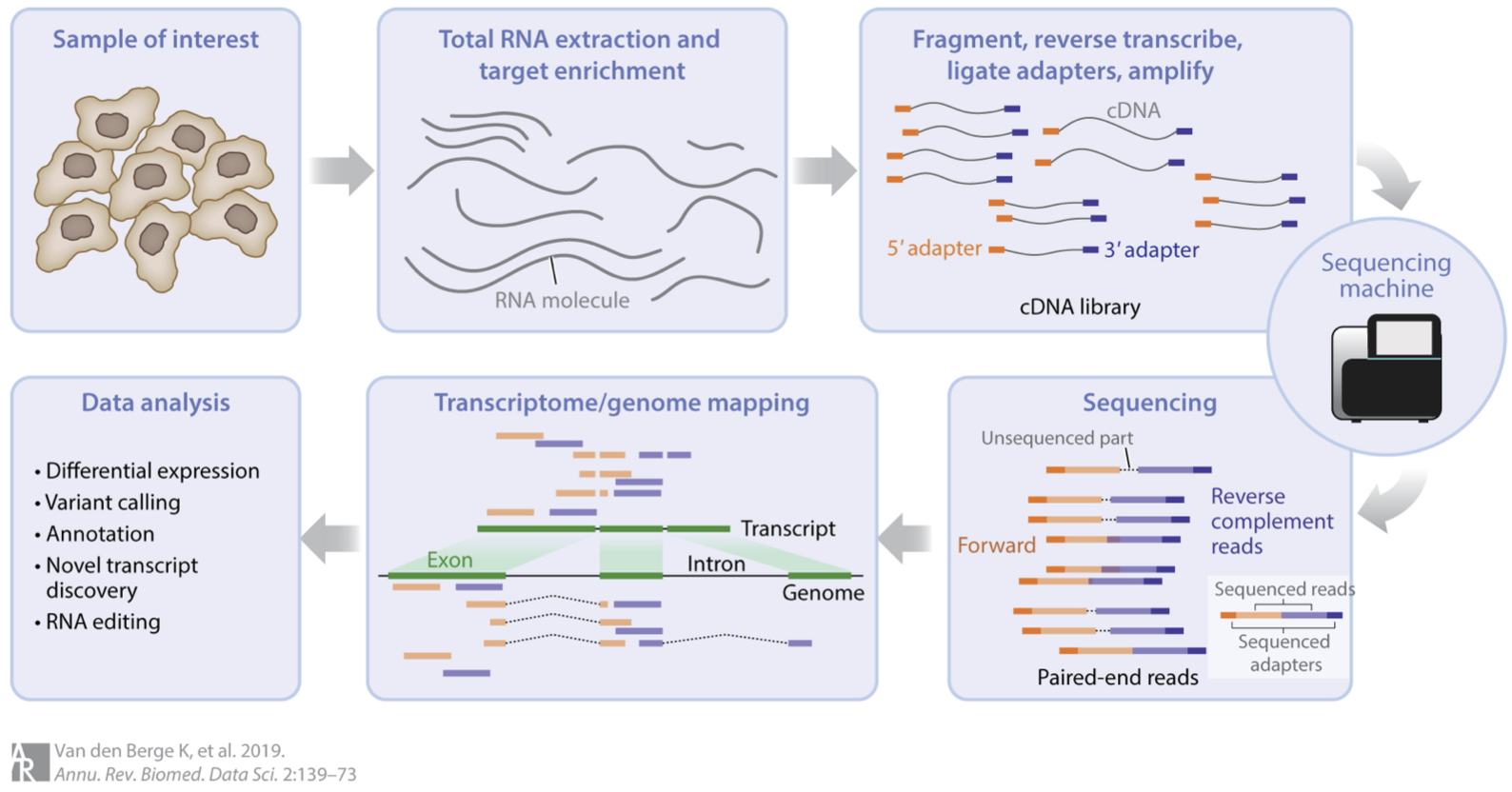
We could say a lot more about each step, but this isn’t our focus. For us, the important thing to know is that after this whole process we arrive at a table of counts—the fundamental object of RNA-seq data analysis. For example, here’s a made up table of counts for two groups (A and B) each with three biological replicates (using the typical ‘genes rows, samples in columns’ convention):
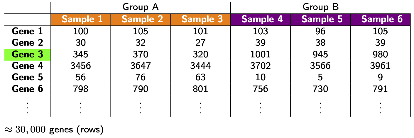
The counts quantify expression: more counts, more expression (roughly speaking—see below). The fundamental question we want to ask is: which genes are DE between the groups? (e.g. is Gene 3 DE?)
Before proceeding, some important comments about replicates:
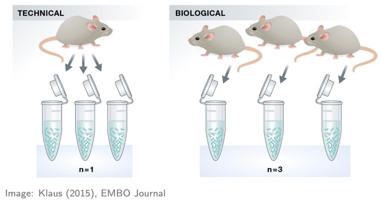
- If you don’t have replicates (ideally for all groups), STOP! You’ll likely produce rubbish results (actually statistical tools will often give you an error in this situation, but not always!). Here “replicates” means biological replicates (data collected from distinct individuals), not technical replicates (data repeatedly collected from the same individual), a distinction nicely depicted in the figure below. Biological replicates are essential because you cannot do rigorous RNA-seq analysis (i.e. statistics) without them. Why? There are many reasons, e.g. you’ll have no way of estimating the (biological) variation, i.e. “noise”, in your data and so no way of properly comparing any “signal” (of DE) to the “noise” (actually there are some ways around this issue but they’re not recommended). Thus, 2 replicates is a minimum and 3+ replicates (depending on the context and situation) are recommended.
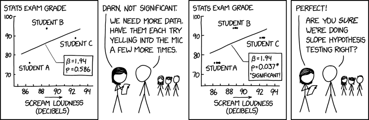
- If you have technical replicates, PROCEED CAREFULLY! They shouldn’t be analysed as if they were separate (independent) samples. Why? To see the main reason, consider an example: suppose one of your groups consists of three individuals each with 2 technical replications, making 3x2 = 6 samples in that group. It may seem like there’s 6 samples in that group for doing the relevant statistics, but don’t be fooled: there’s only 3 independent samples (i.e. distinct individuals). If you analysed the 6 samples as if they were separate samples, your analysis would “overestimate” the amount of information available—there’s only 3 “pieces” of information, not 6—and thus might produce many false discoveries (because the estimated variation might be too small). The standard advice for handling technical replicates is this: add the counts (gene-wise) of each technical replicate to produce single biological replicates. Note, however, that this only applies if there’s no significant technical differences between the replicates (e.g. the technical replicates sit almost on top of each other in a PCA plot—see below). If there are significant technical differences between the replicates (e.g. if each replicate is in different batch, which incidentally is one of the main reasons for generating technical replicates) then you should consult an expert. And, if you’re in doubt about applying this advice, consult an expert!
Another nice way of understanding the technical replicate issue above is through humour, e.g. reflect on the mistake being made in this xkcd comic:
Example data
For illustration, we’ll look at data from the publication: Obers et al. “Retinoic acid and TGF-β orchestrate organ-specific programs of tissue residency”, Immunity (2024). The aim of this study was to investigate the roles of retinoic acid (RA) and the cytokine TGFb in driving organ-specificity of tissue resident T cells.
The relevant RNA-seq counts table for this study can be obtained from Gene Expression Omnibus as follows:
- Use this link
- Scroll down to the “Supplementary file” section
- For the file “GSE232852_CountsTable.txt.gz” (first row), hit “ftp” or “http” in the “Downloads” column
Once the file is downloaded, move it to your R working directory and unzip it. Now let’s read it into R and take a look (note: you’ll need to adjust the file path accordingly):
R
tab <- read.table("data/GSE232852_CountsTable.txt", header=TRUE)
head(tab, n=50)
OUTPUT
            EnsemblID        Symbol RA_1 RA_2 RA_3 TGFb_1 TGFb_2 TGFb_3
1  ENSMUSG00000102693 4933401J01Rik    0    0    0      0      0      0
2  ENSMUSG00000064842       Gm26206    0    0    0      0      0      0
3  ENSMUSG00000051951          Xkr4    0    0    0      0      0      0
4  ENSMUSG00000102851       Gm18956    0    0    0      0      0      0
5  ENSMUSG00000103377       Gm37180    0    0    0      0      0      0
6  ENSMUSG00000104017       Gm37363    0    0    0      0      0      0
7  ENSMUSG00000103025       Gm37686    0    0    0      0      0      0
8  ENSMUSG00000089699        Gm1992    0    0    0      0      0      0
9  ENSMUSG00000103201       Gm37329    0    0    0      0      0      0
10 ENSMUSG00000103147        Gm7341    0    0    0      0      0      0
11 ENSMUSG00000103161       Gm38148    0    0    0      0      0      0
12 ENSMUSG00000102331       Gm19938    0    0    0      0      0      0
13 ENSMUSG00000102348       Gm10568    0    0    0      0      0      0
14 ENSMUSG00000102592       Gm38385    0    0    0      0      0      0
15 ENSMUSG00000088333       Gm27396    0    0    0      0      0      0
16 ENSMUSG00000102343       Gm37381    0    0    0      0      0      0
17 ENSMUSG00000102948        Gm6101    0    0    0      0      0      0
18 ENSMUSG00000025900           Rp1    0    0    0      0      0      0
19 ENSMUSG00000104123       Gm37483    0    0    0      0      0      0
20 ENSMUSG00000025902         Sox17    0    0    0      0      0      0
21 ENSMUSG00000104238       Gm37587    0    0    0      0      0      0
22 ENSMUSG00000102269        Gm7357    2    0    1      0      0      0
23 ENSMUSG00000096126       Gm22307    0    0    0      0      0      0
24 ENSMUSG00000103003       Gm38076    0    0    0      0      0      0
25 ENSMUSG00000104328       Gm37323    0    0    0      0      0      0
26 ENSMUSG00000102735        Gm7369    0    0    0      0      0      0
27 ENSMUSG00000098104        Gm6085   16   30   10     16     14     10
28 ENSMUSG00000102175        Gm6119    0    2    1      1      3      0
29 ENSMUSG00000088000       Gm25493    0    0    0      0      0      0
30 ENSMUSG00000103265        Gm2053    0    0    0      1      1      1
31 ENSMUSG00000103922        Gm6123   10   11    6      2      5      4
32 ENSMUSG00000033845        Mrpl15  948 1158  880    940    880    943
33 ENSMUSG00000102275       Gm37144    9   21   19     12      4      6
34 ENSMUSG00000025903        Lypla1  609  711  577    752    688    647
35 ENSMUSG00000104217       Gm37988    1    3    1      0      3      2
36 ENSMUSG00000033813         Tcea1 1289 1617 1252   1427   1270   1216
37 ENSMUSG00000062588        Gm6104    1    2    2      2      3      3
38 ENSMUSG00000103280       Gm37277    0    0    0      0      0      0
39 ENSMUSG00000002459         Rgs20    0    0    0      2      0      0
40 ENSMUSG00000091305       Gm17100    0    0    0      0      0      0
41 ENSMUSG00000102653       Gm37079    0    0    0      0      0      0
42 ENSMUSG00000085623       Gm16041    0    0    0      0      0      0
43 ENSMUSG00000091665       Gm17101    0    0    0      0      0      0
44 ENSMUSG00000033793       Atp6v1h  873 1047  756   1110   1024   1009
45 ENSMUSG00000104352        Gm7182    0    0    0      0      0      0
46 ENSMUSG00000104046       Gm37567    0    0    0      0      0      0
47 ENSMUSG00000102907       Gm38264    0    0    0      0      0      0
48 ENSMUSG00000025905         Oprk1    0    0    0      0      0      0
49 ENSMUSG00000103936       Gm36965    0    0    0      0      0      0
50 ENSMUSG00000093015       Gm22463    0    0    0      0      0      0
   RA_TGFb_1 RA_TGFb_2 RA_TGFb_3 WT_1 WT_2 WT_3
1          0         0         0    0    0    0
2          0         0         0    0    0    0
3          0         0         0    0    0    0
4          0         0         0    0    0    0
5          0         0         0    0    0    0
6          0         0         0    0    0    0
7          0         0         0    0    0    0
8          0         0         0    0    0    0
9          0         0         0    0    0    0
10         0         0         0    0    0    0
11         0         0         0    0    0    0
12         0         0         0    0    0    0
13         0         0         0    0    0    0
14         0         0         0    0    0    0
15         0         0         0    0    0    0
16         0         0         0    0    0    0
17         0         0         0    0    0    0
18         0         0         0    0    0    0
19         0         0         0    0    0    0
20         0         0         0    0    0    0
21         0         0         0    0    0    0
22         1         0         1    0    0    0
23         0         0         0    0    0    0
24         0         0         0    0    0    0
25         0         0         0    0    0    0
26         0         0         0    0    0    0
27        12        14        16    9   15   19
28         3         4         2    0    0    2
29         0         0         0    0    0    0
30         0         1         0    0    0    0
31         7         9         7    5    4   11
32       656      1197       944 1123  967 1375
33        17        17        18   12    9   24
34       476       837       688  717  709  846
35         0         3         0    0    1    2
36       993      1666      1440 1563 1445 1878
37         2         1         1    5    0    7
38         0         0         0    0    0    0
39         0         0         0    0    0    0
40         0         0         0    0    0    0
41         0         0         0    0    0    0
42         0         0         0    0    0    0
43         0         0         0    0    0    0
44       819      1417      1144 1101  973 1347
45         0         0         0    0    0    0
46         0         0         0    0    0    0
47         0         0         0    0    0    0
48         0         0         0    0    0    0
49         0         0         0    0    0    0
50         0         0         0    0    0    0
Here’s what we have:
- The first 2 columns are gene annotation: “EnsembleID” and “Symbol”, respectively (note: EnsembleID is one of many standard gene identifiers in use; anther common identifier is “Entrez” gene ID).
- The next 12 columns represent the count data on the four experimental groups of interest, each with three biological replicates; specially, a special kind of T cell treated with either: RA, TGFb, both (RA_TGFb), or neither (WT).
Preliminaries
Before we can start analysing this data, there’s four preliminaries:
- Let’s load the R packages we’ll be using (note: if you don’t have the relevant packages installed, then you’ll need to run the commented code):
R
# # CRAN packages
# install.packages(c("ggplot2","ggrepel","ggfortify","scales","pheatmap","matrixStats","openxlsx"))
library(ggplot2)
library(ggrepel)
library(ggfortify)
library(scales)
library(pheatmap)
library(matrixStats)
library(openxlsx)

# # Bioconductor packages
# install.packages("BiocManager")
# BiocManager::install(c("limma","edgeR"))
library(limma)
library(edgeR)
We’ll mainly be using limma and some functions from
edgeR to analyse the data above; the other packages will be
used for plotting and exporting results tables.
- We need to organize our data into
DGEListwhich is a special “container” for our analysis:
R
annotation <- tab[,c(1,2)]
counts <- tab[,-c(1,2)]

dge <- DGEList(counts=counts, genes=annotation)
Note that we split the data table into two distinct parts—gene annotation and counts—storing each into the relevant slots of the container.
- It’s helpful to create a table of sample information:
R
samples <- colnames(tab)[-c(1,2)]
group <- c(rep("RA",3), rep("TGFb",3), rep("RA_TGFb",3), rep("WT",3))

info <- data.frame(samples, group)
info
OUTPUT
     samples   group
1       RA_1      RA
2       RA_2      RA
3       RA_3      RA
4     TGFb_1    TGFb
5     TGFb_2    TGFb
6     TGFb_3    TGFb
7  RA_TGFb_1 RA_TGFb
8  RA_TGFb_2 RA_TGFb
9  RA_TGFb_3 RA_TGFb
10      WT_1      WT
11      WT_2      WT
12      WT_3      WT
Here the first column is a unique sample name and the second labels the experimental group the sample belongs to. Incidentally, this would be the place to store any other relevant sample information (e.g. what batch each sample belongs to, if relevant) and even relevant biological covariates (e.g. sex, age, etc.). Note also that such sample information is usually prepared separately (in, say, Excel) and then read into R; since our example is simple, we created it on the fly.
- We need to create a factor vector for our groups:
R
group <- factor(info$group)
group
OUTPUT
 [1] RA      RA      RA      TGFb    TGFb    TGFb    RA_TGFb RA_TGFb RA_TGFb
[10] WT      WT      WT
Levels: RA RA_TGFb TGFb WT
Factor vectors are special in R: they have an extra piece of
information called “levels” (in this case, it’s saying this factor has
four levels), information which R uses to specify statistical models
etc. As you’ll see, this particular group vector will be
important in our analysis.
- RNA-seq measures gene expression across the transcriptome, producing count data per gene per sample.
- The main goal of DE analysis is to identify genes with expression differences between conditions.
- Biological replicates are required for valid statistical inference; technical replicates must be combined or carefully handled.
- A “counts table” is the starting point for most RNA-seq analyses in R.
- Preparing a DGEList object and sample metadata correctly is essential for downstream analyses with limma and edgeR.
- Understanding the data structure and design factors early helps ensure trustworthy DE results later.